Machine learning in Python with Scikit-learn - a crash course

Or: how to fake your way through machine learning

At my place of work, we recently had a hackathon (during work hours!) in which we could spend 2 days trying to create something that would benefit the company. My idea was to use machine learning for this:

Predicting loan defaults

I would use existing customer data, with knowledge of who did and did not default (i.e. not pay us back), to then predict whether a currently-applying customer would default or not.

My knowledge of machine learning was almost entirely from doing Andrew Ng’s machine learning course on Coursera, but it had been about a year since I’d done it and had never implemented anything afterwards.

So my 2-day hackathon was a bit of a crash course in machine learning. Here’s how I did it:

The basics

This is labelled training. I had a large amount of data (which I obviously cannot share!) with each row containing information that we knew about a customer at their point of application, and whether or not they had defaulted.

This was a classification exercise. That means I was just trying to classify each new customer as predicted to default or not default.

The plan

I used Scikit-Learn, which seems to be a widely-popular library for doing machine learning in Python. It implements a wide range of machine learning algorithms so I would not have to do that work myself. This would be an exercise in plugging things together (I hoped!).

First steps - manipulating data

Scikit-Learn requires all inputs to be numerical. No text, no dates, not even any null/empty fields.

My data was made of mostly publicly available information (e.g. Companies House data) plus information the customer themselves provide. This included plenty of blank fields - for example, newer companies would have less information on Companies House.

Step one then - load in the data.

import pandas as pd

training_path = r'application_info.csv'

# Read in data
df = pd.read_csv(training_path)

Text/string fields

An example text field: industry category

Scikit-Learn won’t take string inputs. But you can’t just convert each string to a number - Scikit-Learn would treat that column as linearly related, but that makes no sense - if you label ‘Transport’ as 1, ‘Television’ as 2, ‘Catering’ as 3 and so on, you’re saying Television is halfway between Transport and Catering - which is meaningless.

Instead, you need to have each industry category be its own column, and set the values to be 1 (for yes, this row is in this category) or 0 (for not).

Scikit-Learn can do this for you, using a LabelBinarizer:

from sklearn.preprocessing import LabelBinarizer

lb = LabelBinarizer()
    
X = lb.fit_transform(df[label].values)
    
# add new generated columns to data
newColumn = pd.DataFrame(X, columns = [label+str(int(i)) for i in range(X.shape[1])])
    df = pd.concat([df, newColumn], axis=1)

# Delete old label, add new ones
features.remove(label)
for i in range(X.shape[1]):
   features.append(label+str(int(i)))

Getting rid of nulls

There are choices to be made here. These are your potential strategies:

• delete rows with nulls. This was impractical for me - I would lose too much data
• Replace nulls with something:
  • 0
  • The mean of the rest of the values in that column
  • The median

Which makes the most sense? It depends on the data. For example, a customer’s total other loans - what does null mean in this instance? Should we assume they don’t have other loans, or just that we’re lacking that information? It’s a choice you have to make.

Whatever you do, you will affect your overall result. It’s best to play around with these (which I’ll discuss later).

Dates

You can do whatever you want here - it might just be easiest to delete dates if they are irrelevant.

I just ignored dates. But if you want to use them, you could extract numerical data from them, e.g. day of the week 1-7, time of day, year etc.

Starting to process data

What algorithm are you going to use? What parameters? How to start?

Scikit-Learn has a pattern which allows you to try a load of things at once, a method called GridSearchCV.

There is a great example of how to use this on my friend George’s Github page

from sklearn.pipeline import Pipeline
from sklearn.linear_model import LogisticRegression
from sklearn.svm import SVC
from sklearn.preprocessing import StandardScaler
from sklearn.model_selection import GridSearchCV

pipeline = Pipeline([
    ('scale', None), 
    ('predict', None)
])

# Set up some parameters
params = [
    {
    'scale':[None, StandardScaler()],
    'predict': [LogisticRegression()],
    'predict__C': [0.1, 1, 10, 100, 1000]
    },
    {
    'scale':[None, StandardScaler()],
    'predict': [SVC()],
    'predict__C': [0.1, 1, 10, 100, 1000]
}
]

gs = GridSearchCV(pipeline, params, scoring='accuracy', cv=StratifiedKFold(), return_train_score=True)
gs.fit(X, y)

print(gs.best_estimator_)

We define some parameters, define the algorithms we want to use, and search every combination of the parameters.

We have also introduced scalers, to scale the data.

This code will score each one based on accuracy (how many predictions were correct) and print the most successful combination of parameters.

Scaling data

Many machine learning algorithms require/prefer data to be scaled - i.e. all data in the same range. Scikit-Learn includes a bunch of scalers, and you can try out what works. I ended up using a MinMaxScaler, scaling all my data to between 0 and 1. This is something to play around with (and your experimentation can be automated, as above).

Scoring

Scoring by accuracy can be a bad idea - and in my case, it was. The % of people who default on loans is pretty small. Imagine it was 5% (not the real value in my data). Then any algorithm which predicts no one to default will score 95% accuracy.

This is exactly what happened to me - very high accuracy, absolutely useless result.

Alternative scoring methods are available.

This one is more useful in the instance where you have very few positive results:

Precision and recall

Precision and recall are alternative ways of evaluating models:

precision = true positives / (true positives + false positives) Conceptually, this means - of the customers I said would default, how many actually did?

recall = true positives / (true positives + false negatives) Conceptually, this means - of the customers who defaulted, how many did I correctly identify?

Example: 35 people default. You predict 50 will default, of which 25 are correctly identified and 25 are falsely accused. You also miss 10 defaulters, who you mark as good customers. Precision = 25 / (25 + 25) = 50% Recall = 25 / (25 + 10) = 71%

For further reading: Toward Science blog

F1 score

The F1 score tries to balance precision and recall, so is very useful in this case - and indeed in any case where your distribution of results is not evenly weighted.

Confusion matrix

A confusion matrix can be a really great way of visualising how your model is doing.

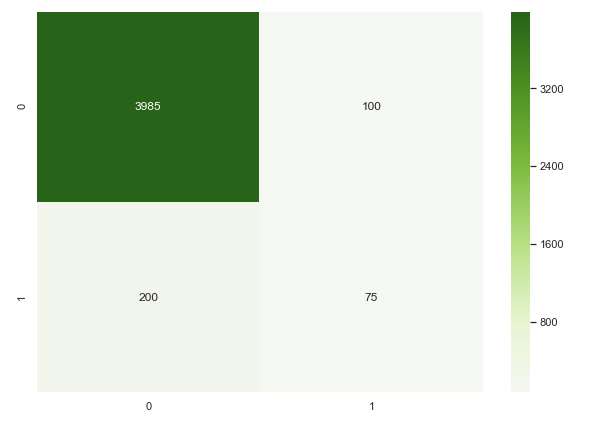
When using a confusion matrix, your aim is to maximise the numbers in the top left and bottom right - these are your true negatives and true positives. The bottom left and top right represent mis-categorised customers, so should be minimised.

In our case, we start by assuming no one defaults (before starting this project). Therefore all our customers are on the left - the right side of the matrix contains no one.

Our aim is to move as many people as possible from the bottom left (people who you say are good customers but actually default) to the bottom right (number of people you correctly identify as being defaulters) without increasing the number in the top right (number of people you accuse of being defaulters who are not).

You can get a text confusion matrix by comparing your test results with your test predictions:

from sklearn.metrics import confusion_matrix

matrix = confusion_matrix(y_test, y_pred)
print (matrix)

And draw an image as I have done like this:

import matplotlib.pyplot as plt
import numpy as np
import seaborn as sns
sns.set()

df_cm = pd.DataFrame(matrix, index = [i for i in "01"],
                  columns = [i for i in "01"])
plt.figure(figsize = (10,7))
sns.heatmap(df_cm, annot=True, fmt='g', cmap="PiYG", center=1)

train_test_split

To prove what you’re doing is right, you need to split your data into a training section and a test section. You ‘fit’ the algorithm using the training data, and test how well it works using the test data.

Anything else is cheating - you can get very good results by testing against the whole data set, but you cannot learn anything from it - it will not be a good predictor of future unseen data.

Scikit-Learn has a ‘train_test_split’ method which will divide up your data for you (see below).

Putting it all together

Once I’d decided on my algorithm with the most success - a RandomForestClassifier - I put it all together:

from sklearn.impute import SimpleImputer
from sklearn.pipeline import Pipeline
from sklearn.ensemble import RandomForestClassifier
from sklearn.model_selection import train_test_split

# Now do the rest
y = df.Defaulted.values

X = df[features]

columns = X.columns
index = X.index

classifier = RandomForestClassifier(n_estimators = 10)

pipeline = Pipeline(
[
    ('impute', SimpleImputer(missing_values=np.nan, strategy='constant', fill_value=0)),
    ('scale', MinMaxScaler(feature_range=(0, 1))),
    ('predict', classifier)
])

x_train, x_test, y_train, y_test = train_test_split(X,y, test_size= 0.2, random_state=27)

pipeline.fit(x_train, y_train)

# make predictions against test data
y_pred = pipeline.predict(x_test)

So I’ve told Scikit-Learn to impute (fill) missing values with 0, scale all my data to between 0 and 1, and run a RandomForestClassifier with 80% of the data as my training set.

You can then plot a confusion matrix and see how well you’ve done.

Prediction confidence levels

Alternative prediction method:

# make predictions against test data
y_pred = pipeline.predict_proba(x_test)

This will give you the results along with confidence levels of the algorithm. Each ‘prediction’ has an estimate for its confidence of the negative and positive result, e.g. [0.2, 0.8]. These will always add up to 1.

If it’s important to be very confident, you could filter out everything under (for example) 80% confidence.

Conclusion

So that’s it - in 2 days I put together a fairly good estimator for whether someone would default on their loan or not, using the above code.

It doesn’t really require a huge understanding of machine learning, just the basics.

In summary, your key steps:

• Massage data, remove nulls etc
• Scale your data
• Separate out training and test data
• Fit model to training data
• Test model against test data
• Evaluate your results

And that’s it - from a basic understanding of machine learning, but with no experience of using it, you should be able to hack your way through a simple project like this.